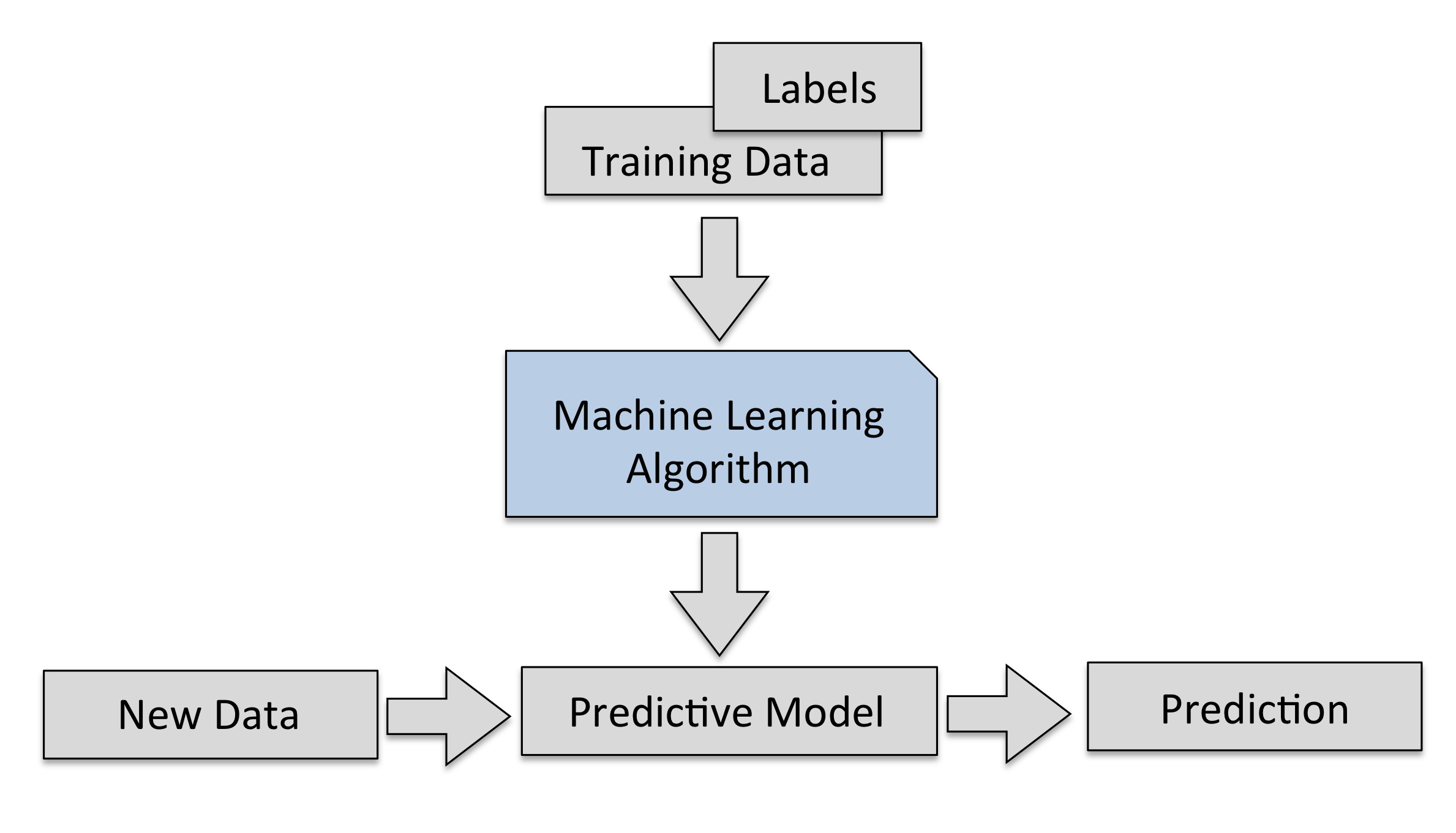
Models
Geometric Models
Geometric models use the concept of instance space The most obvious example of geometric models is when all the features are numerical and can become coordinates in a Cartesian coordinate system. When we only have two or three features they are easy as visualise. However since many machine learning problems have hundreds or thousands of features and therefore dimensions, visualising these spaces is impossible. However many of the geometric concepts, such as linear transformations, still apply in this hyper space.This can help us better understand our models. For instance we expect many learning algorithms will be translation invariant, that is it does not matter where we place the origin in the coordinate system. Also we can use the geometric concept of euclidean distance to measure similarity between instances, this gives us a method to cluster like instances and form a decision boundary between them.
Supposing we are using our linear classifier to classify paragraphs as either happy or sad and we have devised a set of tests. Each test is associated with a weight ,w, to determine how much each test contributes to the overall result.
We can simply sum each test, multiplied by its weight, to get an overall score and create a decision rule that will create a boundary, say if the happy score is greater than a threshold t.

Each feature contributes independently to the overall result, hence the rules linearity. This contribution depends on each features relative weights. These weights can be positive or negative and each individual feature is not subject to the threshold in calculating the overall score.
We can rewrite this sum using vector notation using w for a vector of weights (w1,w2,...,wn) and
x for a vector of test results (x1,x2,...xn). Also if we make it an equality we can define the decision boundary:
w . x = t
We can think of w as a vector pointing between the 'centres of mass' of the positive (happy) examples, P , and the negative examples, N. We can calculate these centres of mass by averaging:

Our aim now is to create a decision boundary half way between these centres of mass. We can see that w is proportional, or equal to, P - N and that (P + N)/ 2 will be on the decision boundary. So we can write :

fig Decision boundary

Insert image B05198_01_08.png
In practice real data is noisy and not necessarily that easily separable. Even when data is easily separable a particular decision boundary may not have much meaning. Consider data that is sparse, such as in text classification where the number of words is large compared to the number of instances of each word. In this large area of empty instance space it may be easy to find a decision boundary but which is the best one? One way is to use a margin to measure the distance between the decision boundary and its closest instance. We will explore these techniques later in the book.
Probabilistic Models
A typical example of a probabilistic model is the Bayesian classifier. Given some training data, D, and a probability based on an initial training set, a particular hypothesis, h, called the posteriori probability, P (h/D).

As an example consider we have a bag of marbles. We know that 40% of them are red and 60% are blue. We also know that of the red marbles half of them have flecks of white and all the blue marbles have flecks. When we reach into the bag to select a marble we can feel by its texture that it has flecks. What are the chances it is red?
Let P(RF) = the probability that a randomly drawn marble with flecks is red.
P(FR) = the probability of a red marble with flecks = 0.5
P(R) = the probability a marble is red = 0.4
P(F) = the probability that a marble has flecks = 0.5 x 0.4 + 1 x 0.6= 0.8

Probabilistic models allow us to allow us to explicitly calculate probabilities, rather than just a binary true or false. As we know the key thing we need to do is create a model that maps or features variable to a target variable. When we take a probabilistic approach we assume there is an underlying random process that creates a well defined, but unknown, probability distribution.
Consider a spam detector. Our feature variables, X, could consist of a set of words that indicate the email might be spam, The target variable Y is the instance class: spam or ham. We are interested in the conditional probability of Y given X. For each email instance there will be a feature vector, X, consisting of boolean values representing the presence of our spam words. We are trying to find Y our target boolean representing spam or not spam.
Now consider that we have two words, x1 and x2 , that constitute our feature vector X. From our training set we can construct a table such as the following:
|
P(Y = spam| x1 , x2) |
P(Y = not spam| x1 , x2) |
|
|
P(Y| x1 = 0, x2 = 0) |
0.1 |
0.9 |
|
P(Y| x1 = 0, x2 = 1) |
0.7 |
0.3 |
|
P(Y| x1 = 1, x2 = 0) |
0.4 |
0.6 |
|
P(Y| x1 = 1, x2 = 1) |
0.8 |
0.2 |
Table 1.1
We can see that once we begin adding more words to our feature vector it will quickly grow unmanageable. With a feature vector of n size we will have 2n cases to distinguish. Fortunately there are other methods to deal with this problem as we shall see later.
The probabilities in the above table are known as posterior probabilities. These are used when we have knowledge from a prior distribution. For instance that one in ten emails is spam. However consider a case where we may know that X contains x2= 1 but we are unsure of the value of x1 This instance could belong in row two where the probability of it being spam is 0.7, or in row 4 where the probability is 0.8. The solution is to average these two rows using the probability of x1 =1 in any instance. That is the probability that a word, x1, will appear in any email, spam or not.
P(Y|x2=1) = P(Y|x1=0,x2=1)P(x1=0) + P(x1=1,x2=1)P(x1=1)
This is called a likelihood function. If we know, from a training set, that : P(x1=1) = 0.1 and therefore P(x1=0) = 0.9. So we can calculate the probability that an email contains the spam word : 0.7 * 0.9 + 0.8 * 0.1 = 0.71
This is an example of a likelihood function: P(X|Y). So why do want to know the probability of X , something we all ready know, conditioned on Y something we know nothing about. A way to look at this is to consider the probability of any email containing a particular random paragraph, say the the 127th paragraph of War and Peace. Clearly this probability is small regardless if the email is spam or not. What we are really interested in is not the magnitude of these likelihoods but their ratio. How much more likely is an email containing a particular combination of words likely to be spam or not spam. These are sometimes called generative models because we can sample across all the variables involved.
We can use Bayes rule to transform between prior distributions and a likelihood function:

P(Y) is the prior probability, how likely is each class before having observed X. Similarly P(X) is the probability without taking into account Y. If we have only two classes we can work with ratios. For instance if we want to know how much the data favours each class.:
If the odds are less than one we assume that the class in the denominator the most likely. If it is greater than one then the class in the enumerator is the most likely. If we use the data from table 1.1 we calculate the following posterior odds.
The likelihood function is important in machine learning because it creates a generative model. If we know the probability distribution of each word in a vocabulary, together with the likelihood of each one appearing in either a spam or not spam email we can generate a random spam email according to the conditional probability P(X|Y = spam).
Logical Models
Logical models are based on algorithms. They can be translated into a set of formal rules that can be understood by humans. For example : if x1 and x2 = 1 then Class Y = spam. These are called decision rules
These logical rules can be organised into a tree structure. In fig we see that the instance space is iteratively partitioned at each branch. The leaves consist of rectangular areas (or hyper rectangles in the case of higher dimensions) representing segments of the instance space. Depending on the task we are solving the leaves are labelled with a class, probability, real number and so on.
Fig Feature tree

Feature trees are very use full in representing machine learning problems, even those that, at first sight , do not appear to have a tree structure. For instance in the Bayes classifier in the previous section we can partition our instance space in to as many regions as there are combinations of feature values. Decision tree models often employ a pruning technique to delete branches that give an incorrect result. In chapter 3 we will look at a number of ways to represent decision trees in python
Note that decision rules may overlap and make contradictory predictions.
They are then said to be logically inconsistent. Rules can also be incomplete in when they do not take in to account all the coordinates in the feature space. There are a number of ways we can address these issues and we will look at these in detail later in the book.
Since tree learning algorithms usually work in a top down manner the first task is to find a good feature to split on at the top of the tree. We need to find a split that will result in a higher degree of purity in subsequent nodes. By purity I mean the degree to which training examples all belong to the same class. As we descend down the tree, at each level we find the training examples at each node increase in purity, that is they increasingly become separated into their own classes until we reach the leaf where all examples belong to the same class.
To look at this another way we are interested in lowering the entropy of subsequent nodes in our decision tree. Entropy, a measure of disorder, is high at the top of the tree (the root) and is progressively lowered at each node as the data is divided up into its respective classes.
In more complex problems, those with larger feature sets and decision rules, finding the optimum splits is sometimes not possible, at least not in acceptable amount of time. We are really interested in creating the shallowest tree to reach our leafs in the shortest path. The time it takes to analyse each node grows exponentially with each additional feature, so the optimum decision tree may take longer to find than actually using a sub optimum tree to perform the task.
An important property of logical models is that they can, to some extent, provide an explanation for their predictions. For example consider the predictions made by a decision tree. By tracing the path from leaf to root we can determine the conditions that resulted in the final result. This is one of the advantages of logical models in that they can be inspected by a human to reveal more about the problem.
Features
In the same way that decisions in real life are only as good as the information available to us, in a machine learning task the model is only as good as its features. Mathematically features are a functions that maps from the instance space to a set of values in a particular domain. In machine learning most measurements we make are numerical therefore the most common feature domain is the set of real numbers. Other common domains include boolean, true or false, or integers, say when we are counting the occurrence of a particular feature, or finite sets such as a set of colours or shapes.
Models are defined in terms of their features. Also single features can be turned into a model, known a s a univariate model. We can distinguishes between two use of features, related to the distinction between grouping and grading.
Firstly we can group our features by zooming into an area in the instance space. Let f be a feature counting the number of occurrences of a word, x1, in an email X. We can set up conditions such as :
f(X) = 0, emails that do not contain x1, , f(X) > 0, emails that contain x1 one or more times and so on. These conditions are called binary splits because they divide the instance space in to two groups. Those that satisfy the condition and those that don't. We can also split the instance space into more than two segments to create non binary splits. For instance where f(X) = 0 ; 0 < F(X) < 5 ; F(X) > 5 and so on.
Secondly we can grade our features, to calculate the independent contribution each one makes to the overall result. Recall our simple linear classifier. The decision rule of the form:

Since this rule is linear each feature makes an independent contribution to the score of an instance. This contribution depends on wi . If it is positive then an positive xi will increase the score. If wi is negative a positive xi decreases the score. If wi is small or zero then the contribution it makes to the overall result is negligible. It can be seen that the features make a measurable contribution to the final prediction.
These two uses of features, as splits (grouping) and predictors (grading) can be combined into one model. A typical example occurs when want to approximate a non linear function say: y sin π x on the interval -1 < x < 1. Clearly simple linear model will not work. Of course the simple answer is to split the x axis into -1 < x 0 and 0 < On each of these segments we can find a reasonable linear approximation.
Fig Using grouping and grading

Insert image B05198_01_10.png
A lot of work can be done improving our models performance by feature construction and transformation. In most machine learning problems the features are not necessarily explicitly available. They need to be construction from raw data sets and then transformed into something our model can make use of. This is especially important in problems like text classification. In our simple spam example we used what is known as a bag of words representation because it disregards the order of the words. However by doing this we loose important information about the meaning of the text.
An important part of feature construction is discretisation. We can sometimes extract more information, or information that is more relevant to our task by dividing features into relevant chunks. For instance supposing our data consists of a list of peoples precise income and we are trying to determine if there is a relationship between financial income and the suburb lived in. Clearly it would be appropriate if our feature set did not consist of precise incomes but ranges of income. Although strictly speaking we loose information, if we choose our intervals appropriately we will not loose information related to our problem, and our model will perform better and give us results that are more easily interpreted.
This highlights the major tasks of feature selection, separating the signal from the noise.
Real world data will invariable contain a lot of information we do not need as well as just plain random noise, and separating the, perhaps small, part of the data that is relevant to our needs is important to the success of our model. It is of course important that we do not throw out information that may be important to us.
Often our features will be non linear, and linear regression may not give us good results. A trick is to transform the instance space itself. Supposing we have data such as that shown in figure below Clearly linear regression only gives us a reasonable fit, shown in the figure on the left. However we can improve this result if we square the instance space, that is we make x = x2 and y = y2 , shown in the figure on the right.
Variance = .92 Variance = .97
Fig Transforming the instance space
Insert image B05198_01_11.png
We can go further and use a technique called the kernel trick. The idea is that we can create a higher dimensional implicit feature space. Pairs of data points are mapped from the raw data set to this higher dimensional space via a specified function, sometimes called a similarity function.
For instance:
Let x1 = (x1, y1) and x2 = (x2, y2)
We create a 2D to 3D mapping:
The points in the 3D space corresponding to the 2D points x1 and x2 are:
and
Now the dot product of these two vectors is:
We can see that by squaring the dot product in the original 2D space we obtain the dot product in the 3D space without actually creating the feature vectors themselves. Here we have defined the kernel k(x1,x2) = (x1 •x2)2. Calculating the dot product in a higher dimensional space is often computationally cheaper and, as we will see, this technique is used quite widely in machine learning from support vector machines (SVM), principle component analysis (PCA) and correlation analysis.
The basic linear classifier we looked at earlier defines a decision boundary w • x = t . The vector, w, is equal to the difference between the mean of the positive example with the mean of the negative examples. p-n. Suppose we have points n= (0,0) and p = (0,1) . Lets assume that we have obtained a positive mean from two training examples p1 = (-1,1) and p2 = (1,1). Therefore we have:
We can now write the decision boundary as:
Using the kernel trick we can obtain the following decision boundary:
With the kernel we defined earlier:
We can now derive the decision boundary:
This is simply a circle around the origin with a radius √t
Using a kernel allows us to classify each new instance by evaluating it paired with each training example, rather than on the mean of positive and negative example as is the case for the basic linear classifier. This allows us to create more flexible, non linear, decision boundaries.
A very interesting and important aspect is the interaction between features. One form of interaction is correlation. For example words in a blog post, where we perhaps might expect there to be positive correlation between the words 'winter' and 'cold', and a negative correlation between winter and hot. What this means for your model depends on your task. If you are doing a sentiment analysis, you might want to consider reducing the weights of each word if they appear together, since the addition of another correlated word would be expected to contribute marginally less weight to the over all result than if that word appeared by itself.
Also with regards to sentiment analysis we often need to transform certain features to capture their meaning. For example the phrase 'not happy' contains a word that would, if we just used 1-grams, contribute to a positive sentiment score when its sentiment is clearly negative. A solution, apart from using 2-grams which may unnecessarily complicate the model, would be to recognise when these two words appear in a sequence and create a new feature 'not_happy' with an associated sentiment score.
Selecting and optimising features is work well spent. It can be a significant part of the design of learning systems. This iterative nature of design flips between two phases. Firstly understanding the properties of the phenomena you are studying and secondly testing your ideas with experimentation. This experimentation gives us deeper insight into the phenomena, allow us to optimise our features, gain deeper understanding and so on until we are satisfied our model gives us an accurate reflection of reality.
Summary
So far we have introduced a broad cross-section of machine learning problems, techniques and concepts. Hopefully by now you have an idea about how to begin tackling a new and unique problem by breaking it up into its components. We have reviewed some of the essential mathematics and explored ways to visualise our designs. We can see that the same problem can have many different representations and each one may highlight different aspects. Before we can begin modelling we need a well defined objective phrased in terms of a specific, feasible and meaningful question. We need to be clear how we can phrase the question in a way a machine can understand.
We have seen that the design process, although consisting of different, distinct activities, is not necessarily a linear process, but more an iterative one. We cycle through each particular phase, proposing and testing ideas until we feel can jump to the next phase. Sometimes we may jump back to a previous stage. We may sit at an equilibrium point, waiting for a particular event to occur, we may cycle through stages, or go through several stages in parallel.
One of the most important components of a machine learning system is its data. In the same way humans learn by interpreting sensory information, a machine learn from the information retrieved from data. Data varies hugely in quality, availability and type. In many machine learning projects most of the time can be spent collecting, verifying and 'massaging' data in to a shape that is acceptable to our learning algorithms. In the next chapter we will look at the details of this vitally important aspect of machine learning.
Linear Programming
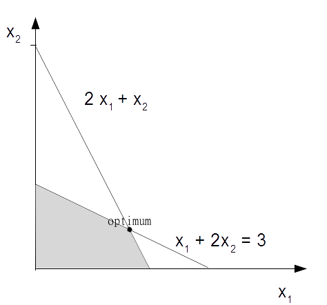
Why are linear models so ubiquitous? Firstly they are relatively easy to understand and implement. They are based on a well founded mathematical theory, developed around the mid 1700's and later played a pivotal role in the development of the digital computer. Computers are uniquely tasked implement linear programs because computers were conceptualised largely on basis of the theory of linear programming. Linear functions are always convex meaning it has only one minima. Linear programming (LP) problems are usually solved using the simplex method. Suppose we want to solve the optimisation problem:
max x1 + x2 with constraints: 2x1 + x2 ≤ 4 and: x1 + 2x2 ≤ 3
We assume x1 and x2 are greater than or equal to 0. The first thing we need to do is convert it to the standard form. This is done by ensuring the problem is a maximisation problem, that is convert min z to max - z. We also need to convert the inequalities to equalities by adding non negative slack variables. The example here already a maximisation problem so we can leave our objective function as it is. We do need to change the inequalities in the constraints to equalities:
2x1 + x2 + x3 = 4 and : x1 + 2x2 + x4 = 3
If we let z denote the value of the objective function we can then write:
z – x1 – x2 = 0
We now have the following system of linear equations.
Objective: z – x1 – x2 + 0 + 0 = 0
Constraint 1: 2x1 + x2 + x3 + 0 = 4
Constraint 2: x1+ 2x2 + 0 + x4 = 3
Our objective is to maximise z remembering that all variables are non negative. We can see that x1 and x2 appear in all the equations and are called non basic. x3 and x4 only appear in one equation each. They are called basic variables. We can find a basic solution by assigning all non basic variables to 0. Here this gives us:
x1 = x2 = 0 ; x3 = 4 ; x4 = 3 ; z = 0.
Is this an optimum solution remembering that our goal is to maximise z? We can see that since z subtracts x1 and x2 in the first equation in our linear system we are able to increase these variables. If the coefficients in this equation were all non negative then there would be no way to increase z. Remember x1 ≥ 0, x2 ≥ 0, x3 ≥ 0 , x4 ≥ 0. So we will know that we have found an optimum solution when all coefficients in the objective equation are positive.
This is not the case here. So we take one of the non basic variables with a negative coefficient in the objective equation, say, x1, called the entering variable, and use a technique called pivoting to turn it from a non basic to a basic variable. At the same time we will change a basic variable, called the leaving variable, into a non basic. We can see that x1 appears in both the constraint equations so which one do we choose to pivot? Remembering we need to keep the coefficients positive. We find that by using the pivot element that yield the lowest ratio of right hand side of the equations to their respective entering coefficients then we can find another basic solution. For x1 in this example this gives us 4/2 for the first constraint and 3/1 for the second. So we will pivot using x1 in constraint 1.
We divide constraint one by 2 and this gives:
x1 + ½ x2 + ½x3 = 2
We can now write this in terms of x1 and substitute it into the other equations to eliminate x1 from these equations. Once we have performed a bit of algebra we end up with the following linear system.
z – 1/2x2 + 1/3 x3 = 2
x1 + 1/2 x2 + 1/2x3 = 2
3/2x2 – 1/2x3 + x4 = 1
We have another basic solution. Is this the optimal solution? Since we still have a minus coefficient in the first equation, the answer is no. We can now go through the same pivot process with x2 and using the ratio rule we find we can pivot on 3/2x2 in the third equation. This gives us:
z + 1/3x3 + 1/3x4 = 7/3
x1 + 2/3x3 – 1/3 x4 = 5/3
x2 – 1/3x3 + 2/3 x4 = 2/3
This gives us the solution of x3 = x4 = 0 ; x1 = 5/3 ; x2 = 2/3 ; and z = 7/3. This is the optimal solution because there are no more negatives in the first equation.
We can visualise this with a graph. The shaded area is the region where we will find a feasible solution.
Design Principles
Design Principles
An analogy is often made between systems design and designing other things such as a house. To a certain extent this analogy holds true. We are attempting to place design components into a structure that meets a specification. The analogy breaks down when we consider their respective operating environments. It is generally assumed in the design of a house that the landscape, once suitably formed, will not change.
Software environments are slightly different. Systems are interactive and dynamic. Any system we design will be nested inside other systems, either electronic, physical, or human. In the same way, the different layers in computer networks (application layer, transport layer, physical layer etc) nest different sets of meanings and function, so as to do activities we do at different levels of a project.
As the designer of these systems we must also have a strong awareness of the setting, the domain in which we work. This knowledge gives us clues to patterns in our data and helps us give context to our work.
Machine learning projects can be divided into 5 distinct activities.
- Defining the object and specification
- Preparing and exploring the data
- Model building
- Implementation
- Testing
- Deployment
The designer is mainly concerned with the first three. However they often play, and in many projects, must play a major role in other activities. It should also be said that a projects timeline is not necessarily a linear sequence of these activities. The important point is that they are distinct activities. They may occur in parallel with each other, and in other ways interact, but they generally involve different types of tasks that can be separated out in terms of human and other resources, stage of the project and externalities. Also we need to consider that different activities involve distinct operational modes. Consider the different ways your brain works when you are sketching out an idea compared to when you are working on a specific analytical task, say a piece of code.
Often the hardest question is where to begin? We can start drilling into the different elements of a problem, with an idea of a feature set, and perhaps an idea of the model or models we might use. This may lead to a defined object and specification, or we may have to do some preliminary research, such as checking possible data sets and sources, or available technologies or to talk to other engineers and technicians and users of the system. We need to explore the operating environment and various constraints, is it part of a web application, or a laboratory research tool for a scientists?
In the early stages of design, our work flow will flip between working on the different elements. For instance we start with a general problem, perhaps having an idea of the task, or tasks, necessary to solve it, then divide it into what we think are key features, try it out on a few models with a toy data set, go back to refine the feature set, adjust our model, and precisely define tasks, refine the model. When we feel our system is robust enough we can test it out on some real data. Of course then we may need to go back, change our feature set...
Selecting and optimising features is often a major activity (really a task in itself) for the machine learning designer. We cannot really decide what features we need until we have adequately described the task, and of course both the task and features are constrained by the types of feasible models we can build.
Types of questions
As designers we are asked to solve a problem. We are given some data and an expected output, a solution. The first step is to frame the problem in a way that a machine can understand and in a way that carries meaning for a human. There are the following six broad approaches we can take to precisely defining our machine learning problem.
- 1.Exploratory: Here we are analysing data looking for patterns, such as a trend or relationship between variables. Exploration often will lead to a hypothesis such as linking diet with disease, or crime rate with suburb.
- 2.Descriptive: Here we are trying to summarise specific features of our data. For instance, the average life expectancy, average temperature or number of left handed people in a population.
- 3.Inferential: An inferential question is one that attempts to support a hypothesis, for instance proving (or disproving) a general link between life expectancy and income by using different data sets.
- 4, Predictive: Here we are trying to anticipate future behaviour. For instance predicting life expectancy by analysing income.
- 5.Casual: his is an attempt to find what causes something. Does low income cause a lower life expectancy?
- 6. Mechanistic: This tries to answer questions like 'what are the mechanisms that link income with life expectancy?'
Most machine learning problems involve several of these types of questionings during development. For instance we may first explore the data looking for patterns or trends, then we may describe certain key features of our data. This may enable us to make a prediction, find a cause or a mechanism behind a particular problem.
Are you asking the right question?
The question must be plausible and meaningful in its subject area. This domain knowledge enables you to understand the things that are important in your data, and see where a certain pattern or correlation has meaning.
The question should be as specific as is possible while still giving a meaningful answer. It is common for it to begin as a generalised statement, such as 'I wonder if wealthy means healthy'. So you do some further research and find you can get statistics for wealth by geographic region, say from the tax office. We can measure health by its inverse, illness, say by hospital admissions and test our initial proposition 'Wealthy means healthy' by tying illness to geographic region. We can see that a more specific question relies on several, perhaps questionable, assumptions.
We should also consider that our results may be confounded by the fact that poorer people may not have health care insurance so are less likely to attend a hospital despite illness. There is an interaction between what we want to find out and what we are trying to measure. This interaction perhaps hides a true rate of illness. All is not lost however. Because we know about these things then perhaps we can account for them in our model.
We can make things a lot easier by learning as much as we can about the domain we are working in.
You could possibly save yourself a lot of time by checking that the question you are asking, or part of it, has not already been answered, or that there are data sets available that may shed some light. Often you have to approach a problem from several different angles at once. Do as much preparatory research as you can. It is quite likely that other designers have done work that could shed light on your own.
Tasks
A task is a specific activity conducted over a period of time. We have to distinguish between the human tasks, planning designing, implementing, to the machine tasks, classification, clustering, regression, and so on. Also consider when there is overlap between human and machine as, say, in selecting features for a model. Our goal really, in machine learning, is to transform as many of these tasks as we can, from human tasks to machine tasks.
It is not always easy to match a real world problem to a specific task. Many real world problems may seem to be conceptually linked, but require a very different methods to solve. Alternatively problems that appear completely different may require similar methods. Unfortunately there is no simple look up table to match a particular task to a problem. A lot depends on the setting and domain. A similar problem in one domain may be unsolvable in another, perhaps because of lack of data. There are however a small number of tasks that are applied to a large number of methods to solve many of the most common problem types. In other words in the space of all possible programming tasks there is a subset of tasks that are useful to our particular problem. Within this subset there is a smaller subset of tasks that are easy and can actually be applied usefully to our problem.
Let’s first briefly introduce the basic machine tasks. Classification is probably the most common type of task, due in part because it is relatively easy, well understood and solves a lot of common problems. Multi class classification (for instance handwriting recognition) can sometimes be achieved by chaining binary classification tasks, however we lose information this way, and we become unable to define a single decision boundary. For this reason multi class classification is often treated separately to binary classification.
There are cases where what we are interested in is not discrete classes but a real number, for instance a probability. These type of problems are regression problems. Both classification and regression require a training set of correctly labelled data. They are supervised learning problems.
Clustering, on the other hand, the task of grouping items without any information on that group is an unsupervised learning task. Clustering is basically making a measurement of similarity.
Related to clustering is association, this is unsupervised task to find a certain type of pattern in a data. This task is behind movie recommender systems, and 'customers who bought this also bought ..' on checkout pages of online stores.
From these basic machine tasks there are a number of derived tasks. In many applications this may simply be applying the learning model to a prediction to establish a casual relationship. We must remember that explaining and predicting are not the same. A model can make a prediction but unless we know explicitly how it made the prediction we cannot begin to form a comprehensible explanation. An explanation requires human knowledge of the domain.
We can also use a prediction model to find exceptions from a general pattern Here we are interested in the individual cases that deviate from the predictions. This is often called anomaly detection and has wide applications in things like detecting bank fraud, noise filtering, even in the search for extraterrestrial life.
An important and potentially useful task is subgroup discovery. Our goal here is not, as in clustering, to partition the entire domain but rather find a subgroup that has a substantially different distribution. In essence subgroup discovery is trying to find relationships between a dependant, target variable an many independent explaining variables. We are not trying to find a complete relationship rather a group of instances that are different in ways that are important in the domain. For instance establishing a subgroup 'smoker = true' and 'family history =true' for a target variable of 'heart disease =true'.
Finally we consider control type tasks. These act to optimise control setting to maximise a pay off given different conditions. This can be achieved in several ways. We can clone expert behaviour, the machine learns directly from a human and makes predictions of actions given different conditions. The task is to learn a prediction model for the experts actions. This is similar to reinforcement learning where the task is to learn a relationship between conditions and optimal action.
Errors
In machine learning systems, software flaws can have very serious real world consequences, what happens if your algorithm embedded in an assembly line robot classifies a human as a production component. Clearly in critical systems you need to plan for failure. There should be a robust fault and error detection procedure embedded in your design process and systems.
Sometimes it is necessary to design quite complex systems simply for the purpose of debugging and checking for logic flaws. It may be necessary to generate data sets with specific statistical structure, or create 'artificial humans' to mimic an interface. For example, developing a methodology to verify that the logic of your design is sound at the data, model, and task levels. Errors can be hard to track, and as a scientist, you must assume there are errors and try to prove your hypothesis.
The idea of recognising and gracefully catching errors is important for the software designer, but as machine learning systems designers we must take it a step further. We need to be able to capture, in our models, the ability to learn from an error.
Consideration must be given to how we select our test set and in particular how representative it is of the rest of the data set. For instance if it is noisy compared to the training set, it will give poor results on the test set suggesting our model is over fitting, when in fact this is not the case. To avoid this a process of cross validation is used. This works by randomly dividing the data into, for example ten chunks of equal size. We use nine chunks for training the model and one for testing. We do this 10 times, using each chunk once for testing. Finally we take an average of test set performance. Cross validation is used with other supervised learning problems besides classification, but, as you would expect, unsupervised learning problems need to be evaluated differently.
Since with an unsupervised task, we do not have a labelled training set. Evaluation can therefore be a little more tricky since we do not know what a correct answer looks like. In a clustering problem for instance we can compare the quality of different models by measures such as the ratio of cluster diameter compared with the distance between clusters. However in problems of any complexity we can never tell if there is another model not yet built, that is better.
Optimisation
Optimisation problems are ubiquitous in many different domains from finance, business, management, sciences, mathematics and engineering. Optimisation problems consist of:
- An objective function that we want to maximise or minimise,
- Decision variables, a set of controllable inputs. These inputs are varied within the specified constraints in order to satisfy the objective function.
- Parameters. These are uncontrollable or fixed inputs
- Constraints. These are relations between decision variables and parameters. They define what values the decision variables can have.
Most optimisation problems have a single objective function. In the cases where we may have multiple objective functions we often find that they conflict with each other, for example reducing costs and increasing output. In practice we try to reformulate multiple objectives into a single function, perhaps by creating a weighted combination of objective functions. In our costs and output example a variable along the lines of cost per unit might work.
The decision variables are the variables we control to achieve the objective. They may include things like resources or labour. The parameters of the module are fixed for each run of the model. We may use several 'cases' where we choose different parameters to test variations in conditions.
There are literally thousands of solution algorithms to the many different types of optimisation problems. Most of them involve first finding a feasible solution, then iteratively improving on this ,by adjusting the decision variables, to, hopefully, find an optimum solution. Many optimisation problems can be solved reasonably well with linear programming techniques. They assume that the objective function and all the constraints are linear with respect to the decision variables. Where these relationships are not linear we often use a suitable quadratic function. If the system is non linear then the objective function may not be convex. That is it may have more than one local minima and there is no assurance that a local minima is a global minima.
The Human Interface
The human interface
For those of you, old enough or unfortunate enough to have used early versions of the Microsoft office suite you will probably remember the 'Mr Clippy' office assistant. This feature, first introduced in Office 97, popped up uninvited from the bottom right of your computer screen every time you typed the letters Dear ..' at the beginning of a document, with the prompt ' it looks like you are writing a letter, would you like help with that?”
Mr Clippy, turned on by default in early versions of Office, was almost universally derided by users of the software and could go down in history as one of machine learning’s first big fails. The Smithsonian Magazine called Mr Clippy “one of the worst software design blunders in the annals of computing”.
So why was the cheery Mr Clippy so hated? Clearly the folks at Microsoft, at the forefront of consumer software development, were not stupid, and the idea that an automated assistant could help with day to day office tasks is not necessarily a bad idea. Indeed later incarnations of automated assistants, the best ones at least, operate seamlessly in the background and provide a demonstrable increase in work efficiency. Consider predictive text. There are many examples, some very funny, of where predictive text has gone spectacularly wrong, but the majority of cases where it doesn't fail it goes unnoticed. It just becomes part of our normal work flow.
At this point we need a distinction between error and failure. Mr Clippy failed because it was obtrusive and poorly designed, not necessarily because it was in error i.e. it could make the right suggestion, but chances are you already know that you are writing a letter. Predictive text has a high error rate, i.e. it often gets the prediction wrong, but it does not fail largely because of the way it is designed to fail unobtrusively.
The design of any system that has a 'tightly coupled human interface', to use systems engineering speak, is difficult. Human behaviour, like the natural world in general, is not something we can always predict. Expression recognition systems, natural language processing and gesture recognition technology, amongst other things, all open up new ways of human machine interaction and this has important applications for the machine learning specialist.
Whenever we are designing a system that requires human input we need to anticipate the possible ways, not just the intended ways, a human will interact with the system. In essence what we are trying to do with these systems is to instil in them some understanding of the broad panorama of human experience
In the first years of the web, search engines used a simple system based on the number of times search terms appeared in articles. Web developers soon began gaming the system, by increasing the number of key search terms. Clearly this would lead to keyword arms race and result in a very boring web. The page rank system, measuring the number of quality inbound links, was designed to provide a more accurate search result. Now, of course, modern search engines use more sophisticated, and secret, algorithms.
What is also important for ML designers is that the co-evolution of humans and algorithms has had an important by-product. A huge data resource that is, in many ways, beginning to distil some of the vastness of human experience. The power of algorithms to harvest this resource, to extract knowledge, insights that would not have been possible with smaller data sets, is massive. So many human interactions are now digitised and we are only just beginning to understand and explore the many ways this data can be used.
As a curious example consider the study 'The expression of emotion in 20th century books (Acerbi et al 2013). Though strictly more of a data analysis study, rather than machine learning, it is illustrative for several reasons. Its purpose is to chart, over time, that most non machine like quality, emotion, extracted from books of the 20th century. With access to a large volume of digitised text through project Gutenberg digital library, WordNet (http://wordnet.princeton.edu/wordnet/) and Googles Ngram database (books.google.com/ngrams), the authors of this study were able to map cultural change over the 20th century as reflected in the literature of the time. They did this by mapping trends in the usage of 'mood' words
For this study the authors labelled each word (a 1gram) and associated it with a mood score and the year it was published. We can see that emotion words, such as joy, sadness, fear and so forth can be scored according to the positive or negative mood they evoke. The mood score was obtained from wordnet (wordnet.princeton.edu). Wordnet assigns an affect score to each mood word. Finally the authors simply counted the occurrences of each mood word.
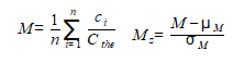
Here ci is the count of a particular mood word, n is the total count of mood words (not all words just words with a mood score). Cthe is the count of the word 'the' in the text. This normalises the sum, to take into account that some years more books were written (or digitised). Also since many later books tend to contain more technical language the word 'the' was used normalize rather than total word count. This gives a more accurate representation of emotion over long time periods in prose text. Finally the score is normalised according to a normal distribution, Mz, by subtracting the mean and dividing by the standard deviation.
Fig From 'The expression of Emotions in 20th Century Books, (Alberto Acerbi, Vasileios Lampos, Phillip Garnett, R. Alexander Bentley) PLOS
Insert image B05198_01_01.png
Here we can see one of the graphs generated by this study. It shows the joy-sadness score for books written in this period and clearly shows a negative trend associated with the period of world war 2.
This study is interesting for several reasons. Firstly it is an example of data driven science, where previously 'soft' sciences such as sociology and anthropology, are given a solid empirical footing. Despite some pretty impressive results, this study was relatively easy to implement. This is mainly because most of the hard work had already been done by wordnet and Google. This highlights how using data resources freely available on the internet and software tools such as the Pythons' data and machine learning packages, anyone one with the data skills and motivation is able build on this work.
Introduction to Machine Learning
In the past decades, many powerful machine learning algorithms have been developed for analyzing data and solving real-world problems. Machine learning systems allow us to utilize the large amounts of data that is available to us in the modern age of technology and help us with decision-making and predictions of future events.
In this chapter, we will learn more about the main concepts and different types of machine learning. Together with a basic introduction to the relevant terminology, we will lay the groundwork to successfully use machine learning techniques for practical problem solving.
In this chapter, we will cover the following topics:
- The general concepts of machine learning
- The three types of learning and basic terminology
- The building blocks to successfully design machine learning systems
- How to install and setup Python for data analysis and machine learning
Building intelligent machines to transform data into knowledge
In this age of modern technology there is one resource that we have in abundance: Large amounts of structured and unstructured data. In the second half of the twentieth century, machine learning evolved as a subfield of artificial intelligence that involves the development of self-learning algorithms to gain knowledge from this data in order to make predictions. Instead of requiring humans to manually derive rules and building models from analyzing large amounts of data, machine learning offers a more efficient alternative to capture knowledge in data for gradually improving the performance of predictive models and making data-driven decisions.
Not only is machine learning becoming increasingly important in computer science research but it also plays an ever-greater role in our everyday life. Thanks to machine learning, we enjoy robust email spam filters, convenient text and voice recognition, reliable web search engines, challenging chess players, and, hopefully soon, safe and efficient self-driving cars.
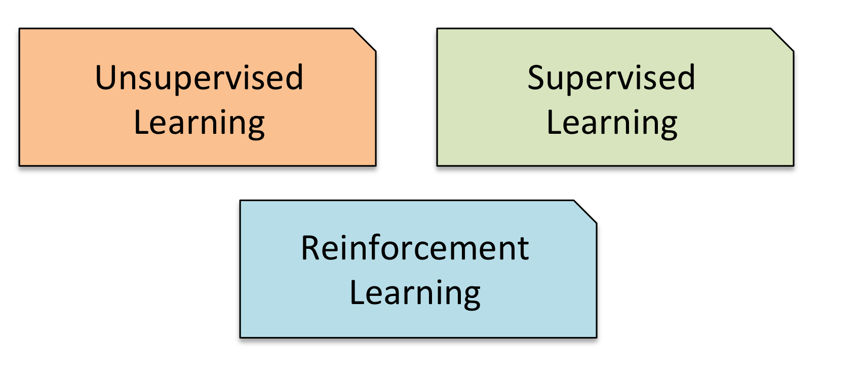
The three different types of machine learning
In this section, we will take a look at the three types of machine learning: Supervised learning, unsupervised learning, and reinforcement learning. We will learn about the fundamental differences between the three different learning types, and using conceptual examples, we will develop an intuition for the practical problem domains where these can be applied.
Making predictions about the future with supervised learning
The main goal in supervised learning is to learn a model from labeled training data that allows us to make predictions about unseen or future data. Here, the term supervised refers to a set training of samples is where the desired output signals (labels) are already known.
Considering the example of email spam filtering, we can train a model using a supervised machine learning algorithm on a corpus of labeled emails to predict whether a new email belongs to the spam or non-spam category. A supervised learning task with discrete class labels, such as in the previous email spam-filtering example, is also called a classification task. Another subcategory of supervised learning is regression where the outcome signal is a continuous value.
Classification for predicting class labels
Classification is a subcategory of supervised learning where our goal is to predict categorical class labels of new instances based on past observations. Those class labels are discrete, unordered values that can be understood as the "group memberships" of the instances. The previously mentioned example of email-spam detection represents a typical example of a binary classification task where the machine learning algorithm learns a set of rules in order to distinguish between two possible classes: spam and non-spam email.
However, the set of class labels does not have to be of binary nature. The predictive model learned by a supervised learning algorithm can assign any class label that was presented in the training dataset to a new, unlabeled instance. A typical example of a multi-class classification task is handwritten character recognition. Here, we could collect a training dataset that consists of multiple handwritten examples of each letter in the alphabet. Now, if a user provides a new handwritten character via an input device, our predictive model would be able to predict the correct letter in the alphabet with certain accuracy. However, our machine learning system would be unable to correctly recognize any of the digits 0 to 9, for example, if they were not part of our training dataset.
The following figure illustrates the concept of a binary classification task given 30 training samples: 15 training samples are labeled as "negative class" (red minus signs) and 15 training samples are labeled as "positive class" (green plus signs). In this scenario, our dataset is 2-dimensional, which means that each sample has two values associated with it, and . Now, we can use a supervised machine learning algorithm to learn a rule – the decision boundary represented as black dashed line – that can separate those two classes and classify new data into each of those two categories given its and values.

Regression for predicting continuous outcomes
We learned in the previous section that the task of classification is to assign categorical, unordered labels to instances. A second type of supervised learning is the prediction of continuous outcomes, which is also called regression analysis. In regression analysis, we are given a number of predictor (explanatory) variables and a continuous response variable (outcome), and we are trying to find a relationship between those variables that allows us to predict an outcome.
For example, let's assume that we are interested in predicting the Math SAT scores of our students. If there is a relationship between the time spent studying for the test and the final scores, we could use it as training data to learn a model that uses the study time to predict the test scores of future students who are planning to take this test.
The term regression was devised by Francis Galton in his article Regression towards mediocrity in hereditary stature in 1886. Galton described the biological phenomenon that the variance of height in a population does not increase over time. He observed that the height of parents is not passed on to their children but the children's height is regressing towards the population mean.
The following figure illustrates the concept of linear regression. Given a predictor variable x and a response variable y, we are fitting a straight line to this data that minimizes the average distance between the sample points and the fitted line. We can now use the intercept and slope learned from this data to predict the outcome variable of new data.

Solving interactive problems with reinforcement learning
Another type of machine learning is reinforcement learning. In reinforcement learning, the goal is to develop a system (agent) that improves its performance based on information that it receives from the environment; this feedback is also called reward signal. Reinforcement learning is related to supervised learning as it receives feedback. However, in reinforcement learning this feedback is not the correct ground truth label or value but a measure of how good the action was measured by a reward function. Through the interaction with the environment, an agent can then use reinforcement learning to learn a series of actions that maximize this reward via an exploratory trial-and-error approach or deliberative planning.
A popular example of reinforcement learning is a chess engine. Here, the agent decides upon a series of moves depending on the state of the board (the environment), and the reward can be defined as "win" or "lose" at the end of the game.

Discovering hidden structures with unsupervised learning
In supervised learning, we know the "right answer" beforehand when we train our model, and in reinforcement learning, we define a measure of reward for particular actions by the agent. In unsupervised learning, however, we are dealing with unlabeled data or data of unknown structure. Using unsupervised learning techniques, we are able explore the structure of our data to extract meaningful information without the guidance of a known outcome variable or reward function.
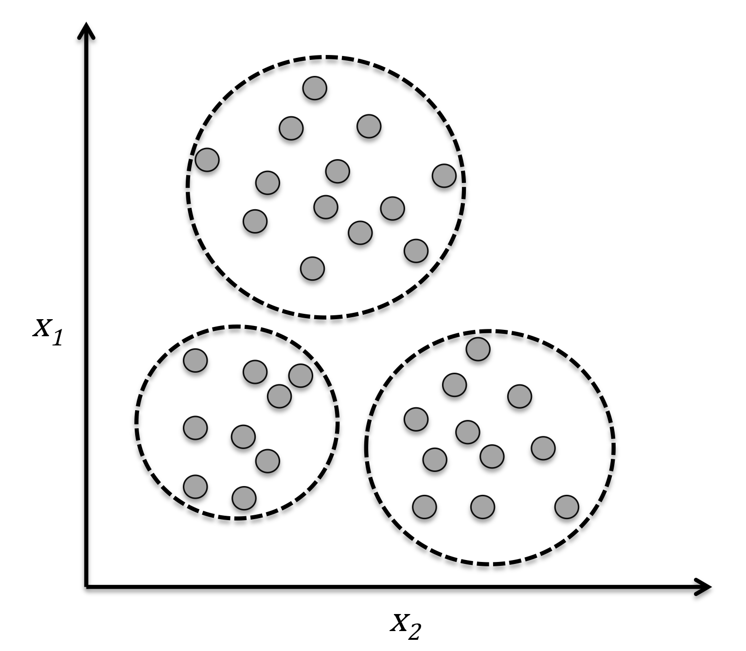
Finding subgroups with clustering
Clustering is an exploratory data analysis technique that allows us to organize a pile of information into meaningful subgroups (clusters) without having any prior knowledge of their group memberships. Each cluster that may arise during the analysis defines a group of objects that share a certain degree of similarity but are more dissimilar to objects in other clusters, which is why clustering is also sometimes called “unsupervised classification.” Clustering is a great technique to structure information and derive meaningful relationships among data, For example, it allows marketers to discover customer groups based on their interests in order to develop distinct marketing programs.
The figure below illustrates how clustering can be applied to organize unlabeled data into three distinct groups based on similarities of their features and .
DMSLdata
Chapter 2
Chapter 3
sampleImage.jpg Right click and save into your ' [working]/data ' directory
