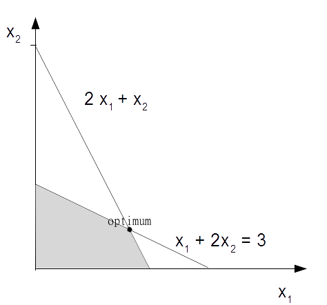
Why are linear models so ubiquitous? Firstly they are relatively easy to understand and implement. They are based on a well founded mathematical theory, developed around the mid 1700's and later played a pivotal role in the development of the digital computer. Computers are uniquely tasked implement linear programs because computers were conceptualised largely on basis of the theory of linear programming. Linear functions are always convex meaning it has only one minima. Linear programming (LP) problems are usually solved using the simplex method. Suppose we want to solve the optimisation problem:
max x1 + x2 with constraints: 2x1 + x2 ≤ 4 and: x1 + 2x2 ≤ 3
We assume x1 and x2 are greater than or equal to 0. The first thing we need to do is convert it to the standard form. This is done by ensuring the problem is a maximisation problem, that is convert min z to max - z. We also need to convert the inequalities to equalities by adding non negative slack variables. The example here already a maximisation problem so we can leave our objective function as it is. We do need to change the inequalities in the constraints to equalities:
2x1 + x2 + x3 = 4 and : x1 + 2x2 + x4 = 3
If we let z denote the value of the objective function we can then write:
z – x1 – x2 = 0
We now have the following system of linear equations.
Objective: z – x1 – x2 + 0 + 0 = 0
Constraint 1: 2x1 + x2 + x3 + 0 = 4
Constraint 2: x1+ 2x2 + 0 + x4 = 3
Our objective is to maximise z remembering that all variables are non negative. We can see that x1 and x2 appear in all the equations and are called non basic. x3 and x4 only appear in one equation each. They are called basic variables. We can find a basic solution by assigning all non basic variables to 0. Here this gives us:
x1 = x2 = 0 ; x3 = 4 ; x4 = 3 ; z = 0.
Is this an optimum solution remembering that our goal is to maximise z? We can see that since z subtracts x1 and x2 in the first equation in our linear system we are able to increase these variables. If the coefficients in this equation were all non negative then there would be no way to increase z. Remember x1 ≥ 0, x2 ≥ 0, x3 ≥ 0 , x4 ≥ 0. So we will know that we have found an optimum solution when all coefficients in the objective equation are positive.
This is not the case here. So we take one of the non basic variables with a negative coefficient in the objective equation, say, x1, called the entering variable, and use a technique called pivoting to turn it from a non basic to a basic variable. At the same time we will change a basic variable, called the leaving variable, into a non basic. We can see that x1 appears in both the constraint equations so which one do we choose to pivot? Remembering we need to keep the coefficients positive. We find that by using the pivot element that yield the lowest ratio of right hand side of the equations to their respective entering coefficients then we can find another basic solution. For x1 in this example this gives us 4/2 for the first constraint and 3/1 for the second. So we will pivot using x1 in constraint 1.
We divide constraint one by 2 and this gives:
x1 + ½ x2 + ½x3 = 2
We can now write this in terms of x1 and substitute it into the other equations to eliminate x1 from these equations. Once we have performed a bit of algebra we end up with the following linear system.
z – 1/2x2 + 1/3 x3 = 2
x1 + 1/2 x2 + 1/2x3 = 2
3/2x2 – 1/2x3 + x4 = 1
We have another basic solution. Is this the optimal solution? Since we still have a minus coefficient in the first equation, the answer is no. We can now go through the same pivot process with x2 and using the ratio rule we find we can pivot on 3/2x2 in the third equation. This gives us:
z + 1/3x3 + 1/3x4 = 7/3
x1 + 2/3x3 – 1/3 x4 = 5/3
x2 – 1/3x3 + 2/3 x4 = 2/3
This gives us the solution of x3 = x4 = 0 ; x1 = 5/3 ; x2 = 2/3 ; and z = 7/3. This is the optimal solution because there are no more negatives in the first equation.
We can visualise this with a graph. The shaded area is the region where we will find a feasible solution.
